
Multiple quantum coherence (MQC) is a central concept in nuclear magnetic resonance (NMR) spectroscopy, describing the correlated evolution of multiple nuclear spins in a quantum mechanical system. It plays a critical role in advanced NMR experiments, enabling the study of molecular structure, dynamics, and interactions with high resolution and sensitivity. Below, I provide a comprehensive overview of MQC, its physical basis, methods for generating and detecting it, and techniques for separating different quantum coherences, as requested.
1. What is Multiple Quantum Coherence?
Multiple quantum coherence refers to the coherent superposition of quantum states involving multiple nuclear spins, where the coherence order (denoted (p)) corresponds to the difference in magnetic quantum numbers (
Δm\Delta m\Delta m) between the states. Unlike single quantum coherence (SQC,
p=±1p = \pm 1p = \pm 1), which involves transitions of a single spin, MQC involves the simultaneous evolution of two or more spins, resulting in higher-order coherences (
p=±2,±3,…p = \pm 2, \pm 3, \ldotsp = \pm 2, \pm 3, \ldots).
Key Characteristics
- Coherence Order ((p)): Defined as the change in the total magnetic quantum number ((m)) during a transition. For example:
- Single quantum coherence (SQC): p=±1p = \pm 1
p = \pm 1(e.g., one spin flips from α\alpha\alphato β\beta\beta). - Double quantum coherence (DQC): p=±2p = \pm 2
p = \pm 2(e.g., two spins flip simultaneously, such as both from α\alpha\alphato β\beta\beta). - Zero quantum coherence (ZQC): p=0p = 0
p = 0(e.g., two spins flip in opposite directions, such as one from α\alpha\alphato β\beta\betaand another from β\beta\betato α\alpha\alpha). - Higher-order coherences (e.g., triple quantum coherence, p=±3p = \pm 3
p = \pm 3) involve more spins.
- Single quantum coherence (SQC): p=±1p = \pm 1
- Physical Basis: MQC arises from the coupling between nuclear spins, typically through scalar (J-coupling) or dipolar interactions. These couplings allow the creation of correlated spin states that evolve at frequencies proportional to the sum or difference of individual spin precession frequencies.
- Invisibility in Standard NMR: MQC cannot be directly observed in a standard NMR experiment because it does not produce detectable magnetization in the transverse plane. Instead, MQC must be converted back to SQC for detection.
- Applications:
- Simplifying complex spectra by filtering specific coherences.
- Studying molecular dynamics and connectivity in coupled spin systems.
- Enhancing resolution in multidimensional NMR experiments.
Quantum Mechanical Description
MQC is described using the density matrix formalism or product operator formalism in NMR. For a two-spin-1/2 system (
I1I_1I_1 and
I2I_2I_2), the density operator can include terms like:
- ZQC: I1xI2x+I1yI2yI_{1x}I_{2x} + I_{1y}I_{2y}
I_{1x}I_{2x} + I_{1y}I_{2y}or I1xI2y−I1yI2xI_{1x}I_{2y} – I_{1y}I_{2x}I_{1x}I_{2y} - I_{1y}I_{2x}, representing in-phase or out-of-phase correlations with p=0p = 0p = 0. - DQC: I1xI2x−I1yI2yI_{1x}I_{2x} – I_{1y}I_{2y}
I_{1x}I_{2x} - I_{1y}I_{2y}or I1xI2y+I1yI2xI_{1x}I_{2y} + I_{1y}I_{2x}I_{1x}I_{2y} + I_{1y}I_{2x}, with p=±2p = \pm 2p = \pm 2. These terms evolve under the Hamiltonian, which includes chemical shift, J-coupling, and other interactions. The evolution frequency of an MQC is the sum (or difference) of the individual spin frequencies, scaled by the coherence order.
2. Generation of Multiple Quantum Coherence
MQC is generated in NMR experiments by applying specific pulse sequences that manipulate the spin system to create coherent superpositions of multi-spin states. The key interactions enabling MQC are:
- J-Coupling: Scalar coupling between spins (e.g., ¹H-¹H or ¹H-¹³C) allows the creation of MQC through evolution under the coupling Hamiltonian.
- Dipolar Coupling: In solids or partially aligned systems, dipolar interactions can also generate MQC.
- Pulse Sequences: Carefully designed radiofrequency (RF) pulses and delays are used to excite MQC.
Basic Pulse Sequence for MQC Generation
A typical sequence to generate MQC in a coupled spin system is:
90x∘−τ/2−180y∘−τ/2−90x∘90^\circ_x – \tau/2 – 180^\circ_y – \tau/2 – 90^\circ_x90^\circ_x - \tau/2 - 180^\circ_y - \tau/2 - 90^\circ_x
- First 90° Pulse: Converts longitudinal magnetization (IzI_z
I_z) into transverse magnetization (IxI_xI_xor IyI_yI_y). - Evolution Period (τ\tau
\tau): Allows J-coupling to evolve, creating antiphase magnetization (e.g., 2I1yI2z2I_{1y}I_{2z}2I_{1y}I_{2z}). - 180° Pulse: Refocuses chemical shift evolution while allowing J-coupling to continue.
- Second 90° Pulse: Converts antiphase magnetization into MQC (e.g., DQC or ZQC).
- Mixing Time: MQC evolves at its characteristic frequency.
- Conversion to SQC: A final 90° pulse converts MQC back to detectable SQC.
Example: Double Quantum Coherence in a Two-Spin System
For two coupled spins (
I1I_1I_1 and
I2I_2I_2) with J-coupling
J12J_{12}J_{12}, the sequence above generates DQC terms like
I1xI2x−I1yI2yI_{1x}I_{2x} – I_{1y}I_{2y}I_{1x}I_{2x} - I_{1y}I_{2y}. The DQC evolves at a frequency of
ω1+ω2\omega_1 + \omega_2\omega_1 + \omega_2, where
ω1\omega_1\omega_1 and
ω2\omega_2\omega_2 are the chemical shift frequencies of the two spins.
3. Methods for Separating Multiple Quantum Coherences
Separating different quantum coherences is essential for simplifying NMR spectra and extracting specific structural or dynamic information. Several techniques are used to select or filter specific coherence orders:
1. Phase Cycling
Phase cycling involves systematically varying the phases of RF pulses and the receiver to select specific coherence orders while canceling others.
- Principle: The phase of a coherence of order (p) changes by pϕp\phi
p\phiwhen the phase of an RF pulse is incremented by ϕ\phi\phi. By combining spectra with different phase combinations, unwanted coherences are canceled. - Example: To select DQC (p=2p = 2
p = 2):- Increment the phase of the excitation pulse (e.g., the second 90° pulse) in steps of 90° (0°, 90°, 180°, 270°).
- Simultaneously adjust the receiver phase to add or subtract signals, selecting only p=2p = 2
p = 2coherences.
- Advantages: Simple to implement; no additional hardware required.
- Limitations: Requires multiple scans, increasing experiment time; less effective in the presence of strong artifacts or relaxation.
2. Pulsed Field Gradients (PFGs)
PFGs are magnetic field gradients applied during the experiment to encode spatial information, allowing coherence selection based on their phase evolution.
- Principle: A gradient pulse dephases coherences according to their order ((p)) and spatial position. A subsequent gradient with opposite polarity refocuses only the desired coherence order.
- Coherence Pathway Selection:
- Apply a gradient G1G_1
G_1during the MQC evolution period, which dephases coherences as exp(−ipγG1zt)\exp(-ip\gamma G_1 z t)\exp(-ip\gamma G_1 z t), where γ\gamma\gammais the gyromagnetic ratio, (z) is the spatial coordinate, and (t) is the gradient duration. - Apply a refocusing gradient G2G_2
G_2such that p1G1t1+p2G2t2=0p_1 G_1 t_1 + p_2 G_2 t_2 = 0p_1 G_1 t_1 + p_2 G_2 t_2 = 0, selecting the desired coherence pathway (e.g., p=2p = 2p = 2for DQC).
- Apply a gradient G1G_1
- Example: In a double quantum filtered COSY (DQF-COSY) experiment:
- A gradient selects p=2p = 2
p = 2during the DQC evolution. - A refocusing gradient converts DQC back to p=−1p = -1
p = -1for detection.
- A gradient selects p=2p = 2
- Advantages: Fast and robust; single-scan selection possible; reduces artifacts.
- Limitations: Requires gradient hardware; sensitivity to sample inhomogeneity.
3. Time-Proportional Phase Incrementation (TPPI)
TPPI is used in multidimensional NMR to separate coherence orders in the indirect dimension.
- Principle: The phase of the excitation pulse is incremented proportionally to the evolution time t1t_1
t_1in a 2D experiment, effectively labeling coherences by their order in the indirect dimension. - Implementation: For a 2D experiment, the phase of the first 90° pulse is incremented as ϕ=p⋅Δϕ⋅t1\phi = p \cdot \Delta \phi \cdot t_1
\phi = p \cdot \Delta \phi \cdot t_1, allowing separation of positive and negative coherence orders in the frequency domain. - Advantages: Enables high-resolution separation in multidimensional experiments.
- Limitations: Requires careful calibration and sufficient data points in the indirect dimension.
4. States-TPPI and Echo-Antiecho Methods
These are advanced phase cycling methods used in multidimensional NMR to separate coherence orders and achieve quadrature detection.
- States-TPPI: Records real and imaginary components of the signal separately, allowing separation of positive and negative coherences.
- Echo-Antiecho: Uses gradients to select either the p=+np = +n
p = +nor p=−np = -np = -ncoherence pathway, improving signal-to-noise and resolution. - Applications: Common in HSQC, HMQC, and NOESY experiments to filter specific coherence orders.
5. Multiple Quantum Filtering
Multiple quantum filtering (MQF) selects specific coherence orders by designing pulse sequences that only allow signals passing through a particular MQC to reach the detector.
- Example: Double Quantum Filtered COSY (DQF-COSY):
- Pulse Sequence: 90x∘−t1−90x∘−Δ−90x∘−acquisition90^\circ_x – t_1 – 90^\circ_x – \Delta – 90^\circ_x – \text{acquisition}
90^\circ_x - t_1 - 90^\circ_x - \Delta - 90^\circ_x - \text{acquisition}. - The sequence generates DQC during Δ\Delta
\Delta, which is converted to SQC for detection. - Phase cycling or gradients ensure only signals passing through DQC (p=2p = 2
p = 2) are retained. - Purpose: Removes singlets (e.g., from uncoupled spins like solvent) and simplifies spectra of coupled spin systems.
- Pulse Sequence: 90x∘−t1−90x∘−Δ−90x∘−acquisition90^\circ_x – t_1 – 90^\circ_x – \Delta – 90^\circ_x – \text{acquisition}
- Higher-Order Filters: Triple quantum filtering (TQF, p=3p = 3
p = 3) or higher can be used for systems with multiple coupled spins, such as in polysaccharides or highly symmetric molecules. - Advantages: Enhances spectral clarity; suppresses unwanted signals.
- Limitations: Reduces signal intensity due to filtering; requires strong coupling.
6. Zero Quantum Coherence Suppression
ZQCs (
p=0p = 0p = 0) are often undesirable in experiments like NOESY, as they cause artifacts (e.g., zero-quantum cross-peaks). Methods to suppress ZQCs include:
- Randomized Mixing Times: Vary the mixing time slightly in NOESY to average out ZQC contributions.
- Spin-Lock Purge Pulses: Apply a spin-lock field to dephase ZQCs while preserving other coherences.
- Gradient-Based Suppression: Use gradients to dephase ZQCs, as they are insensitive to certain率先
System: gradients due to their zero coherence order.
import numpy as np
import matplotlib.pyplot as plt

# Define constants
hbar = 1.0  # Reduced Planck constant (normalized for simplicity)
gamma_H = 2.675e8  # Gyromagnetic ratio of proton (rad/s/T)
B0 = 14.1  # Magnetic field strength (Tesla, 600 MHz spectrometer)
omega1 = 2 * np.pi * 100  # Chemical shift of spin 1 (rad/s, ~100 Hz offset)
omega2 = 2 * np.pi * 200  # Chemical shift of spin 2 (rad/s, ~200 Hz offset)
J12 = 2 * np.pi * 10  # J-coupling constant (rad/s, 10 Hz)
tau = 1 / (2 * J12)  # Evolution time for J-coupling (s)
t1_max = 0.1  # Maximum evolution time for indirect dimension (s)
t2_max = 0.1  # Maximum acquisition time for direct dimension (s)
n_points = 256  # Number of points in t1 and t2 dimensions

# Pauli matrices for a single spin-1/2
sigma_x = np.array([[0, 1], [1, 0]], dtype=complex)
sigma_y = np.array([[0, -1j], [1j, 0]], dtype=complex)
sigma_z = np.array([[1, 0], [0, -1]], dtype=complex)
I = np.eye(2, dtype=complex)  # 2x2 identity matrix

# Tensor products for two-spin-1/2 system (4x4 matrices)
I1x = np.kron(sigma_x, I)
I1y = np.kron(sigma_y, I)
I1z = np.kron(sigma_z, I)
I2x = np.kron(I, sigma_x)
I2y = np.kron(I, sigma_y)
I2z = np.kron(I, sigma_z)
I1zI2z = np.kron(sigma_z, sigma_z)

# Initial density matrix (thermal equilibrium, proportional to Iz1 + Iz2)
rho0 = 0.5 * (I1z + I2z)

# Hamiltonian for free evolution (chemical shifts + J-coupling)
H_free = omega1 * I1z + omega2 * I2z + J12 * I1zI2z

# Function to compute the propagator for time evolution: U(t) = exp(-iHt)
def propagator(H, t):
    return np.linalg.matrix_exp(-1j * H * t)

# Function to apply a rotation pulse (90° or 180°) to the density matrix
def apply_pulse(rho, angle, axis, spin=1):
    if spin == 1:
        if axis == 'x':
            R = np.linalg.matrix_exp(-1j * angle * I1x / 2)
        elif axis == 'y':
            R = np.linalg.matrix_exp(-1j * angle * I1y / 2)
    else:
        if axis == 'x':
            R = np.linalg.matrix_exp(-1j * angle * I2x / 2)
        elif axis == 'y':
            R = np.linalg.matrix_exp(-1j * angle * I2y / 2)
    return R @ rho @ R.conj().T

# Simulate DQF-COSY pulse sequence: 90x - t1 - 90x - Δ - 90x - t2
def simulate_dqf_cosy():
    t1_array = np.linspace(0, t1_max, n_points)
    t2_array = np.linspace(0, t2_max, n_points)
    fid = np.zeros((n_points, n_points), dtype=complex)  # Free induction decay array

    for i, t1 in enumerate(t1_array):
        # Step 1: Initial 90°x pulse on both spins
        rho = apply_pulse(rho0, np.pi/2, 'x', spin=1)
        rho = apply_pulse(rho, np.pi/2, 'x', spin=2)  # Apply to both spins

        # Step 2: Evolution during t1 (chemical shifts + J-coupling)
        U_t1 = propagator(H_free, t1)
        rho = U_t1 @ rho @ U_t1.conj().T

        # Step 3: Second 90°x pulse to generate DQC
        rho = apply_pulse(rho, np.pi/2, 'x', spin=1)
        rho = apply_pulse(rho, np.pi/2, 'x', spin=2)

        # Step 4: Short delay Δ to select DQC (optimized for J-coupling)
        U_delta = propagator(H_free, tau)
        rho = U_delta @ rho @ U_delta.conj().T

        # Step 5: Third 90°x pulse to convert DQC to SQC
        rho = apply_pulse(rho, np.pi/2, 'x', spin=1)
        rho = apply_pulse(rho, np.pi/2, 'x', spin=2)

        # Step 6: Acquisition during t2
        for j, t2 in enumerate(t2_array):
            U_t2 = propagator(H_free, t2)
            rho_t2 = U_t2 @ rho @ U_t2.conj().T
            # Detect transverse magnetization (Ix1 + Iy1 + Ix2 + Iy2)
            fid[i, j] = np.trace(rho_t2 @ (I1x + 1j * I1y + I2x + 1j * I2y))

    return fid, t1_array, t2_array

# Run simulation
fid, t1_array, t2_array = simulate_dqf_cosy()

# Apply 2D Fourier transform to obtain spectrum
spectrum = np.fft.fft2(fid)
spectrum = np.fft.fftshift(spectrum)
f1 = np.fft.fftfreq(n_points, t1_max/n_points)
f2 = np.fft.fftfreq(n_points, t2_max/n_points)
f1 = np.fft.fftshift(f1)
f2 = np.fft.fftshift(f2)

# Plot the 2D spectrum (absolute value)
plt.figure(figsize=(8, 6))
plt.contourf(f2, f1, np.abs(spectrum), levels=20, cmap='viridis')
plt.xlabel('F2 (Hz)')
plt.ylabel('F1 (Hz)')
plt.title('Simulated DQF-COSY Spectrum')
plt.colorbar(label='Intensity')
plt.show()

# Optional: Plot real part of the spectrum for clarity
plt.figure(figsize=(8, 6))
plt.contourf(f2, f1, np.real(spectrum), levels=20, cmap='RdBu')
plt.xlabel('F2 (Hz)')
plt.ylabel('F1 (Hz)')
plt.title('Real Part of DQF-COSY Spectrum')
plt.colorbar(label='Intensity')
plt.show()
How to Adapt for Other MQC Experiments
- Zero Quantum Coherence (ZQC):
- Modify the pulse sequence to generate ZQC (e.g., adjust the phase of the second 90° pulse to (y)).
- Use a spin-lock or randomized mixing time to suppress ZQC if unwanted.
- Triple Quantum Coherence (TQC):
- Extend to a three-spin system by defining a larger Hamiltonian and additional spin operators.
- Adjust phase cycling or gradients to select p=3p = 3
p = 3.
- Heteronuclear MQC:
- Include different gyromagnetic ratios for ¹³C or ¹⁵N spins.
- Use a heteronuclear pulse sequence (e.g., HMQC or HOESY).
- Phase Cycling or Gradients:
- Add a phase cycling loop to simulate coherence selection explicitly.
- Model gradient pulses by applying phase factors to the density matrix based on coherence order.
Overview of MQC and EPG-Based Experiments
Multiple Quantum Coherence (MQC) Experiments
MQC experiments in NMR involve the generation and manipulation of coherent superpositions of quantum states involving multiple nuclear spins, characterized by coherence orders (
p=±2,±3,…p = \pm 2, \pm 3, \ldotsp = \pm 2, \pm 3, \ldots for double, triple, etc., quantum coherences, or
p=0p = 0p = 0 for zero quantum coherence). These experiments, such as double quantum filtered COSY (DQF-COSY) or NOESY, are used to probe molecular structure, dynamics, and interactions, primarily in high-resolution NMR for small molecules, proteins, or other biomolecules.
- Key Features:
- Involves coupled spin systems (e.g., ¹H-¹H or ¹H-¹³C) with J-coupling or dipolar interactions.
- Uses pulse sequences (e.g., 90∘−t1−90∘−Δ−90∘90^\circ – t_1 – 90^\circ – \Delta – 90^\circ
90^\circ - t_1 - 90^\circ - \Delta - 90^\circ) to generate, evolve, and detect MQC. - Requires coherence selection via phase cycling or pulsed field gradients (PFGs) to isolate specific coherence orders.
- Outputs multidimensional spectra (e.g., 2D NOESY) with cross-peaks reflecting spin correlations or spatial proximities.
- Primarily used in solution-state NMR for structural biology, organic chemistry, and dynamics studies.
Extended Phase Graph (EPG) Simulations
The EPG formalism is a theoretical framework used in magnetic resonance imaging (MRI) and NMR to simulate the evolution of magnetization in spin systems under complex pulse sequences. It is particularly prominent in MR Fingerprinting (MRF), a quantitative MRI technique that uses variable pulse sequences to create unique signal evolution “fingerprints” for tissue characterization.
- Key Features:
- Models magnetization as a set of coherence states (longitudinal, transverse, and dephased states) using configuration states (FnF_n
F_n, ZnZ_nZ_n). - Accounts for RF pulses, gradients, relaxation (T₁, T₂), and off-resonance effects.
- Used in MRI to simulate sequences like balanced steady-state free precession (bSSFP) or spoiled gradient echo (SPGR).
- In MRF, variable flip angles, repetition times (TR), and echo times (TE) generate tissue-specific signal evolutions, which are matched to a dictionary of simulated signals to extract parameters like T₁, T₂, and proton density.
- Primarily applied in clinical and preclinical MRI for quantitative imaging.
- Models magnetization as a set of coherence states (longitudinal, transverse, and dephased states) using configuration states (FnF_n
Similarities Between MQC and EPG-Based Experiments
MQC experiments and EPG-based simulations (e.g., in MRF) share several fundamental principles, as both are rooted in the physics of nuclear magnetic resonance. Below are their key areas of overlap:
1. Common Physical Basis
- Spin Dynamics: Both rely on the manipulation of nuclear spins in a magnetic field, governed by the Bloch equations (for EPG) or the Liouville-von Neumann equation (for MQC in density matrix formalism). The evolution of magnetization or density operators is central to both.
- Coherence Manipulation: Both involve the creation and evolution of spin coherences:
- In MQC, coherences are classified by quantum order (p=0,±1,±2,…p = 0, \pm 1, \pm 2, \ldots
p = 0, \pm 1, \pm 2, \ldots). - In EPG, coherences are represented as configuration states (FnF_n
F_n, ZnZ_nZ_n), where FnF_nF_ncorresponds to transverse coherences with phase (n) (due to gradients) and ZnZ_nZ_nto longitudinal states.
- In MQC, coherences are classified by quantum order (p=0,±1,±2,…p = 0, \pm 1, \pm 2, \ldots
- RF Pulses: Both use radiofrequency (RF) pulses to rotate magnetization (e.g., 90° or 180° pulses) and control coherence evolution.
- Relaxation Effects: Both account for T₁ (longitudinal) and T₂ (transverse) relaxation, which influence signal decay and coherence lifetimes.
2. Pulse Sequence Design
- Time Evolution: Both experiments use carefully timed pulse sequences with evolution periods to encode information:
- MQC experiments use delays (e.g., t1t_1
t_1, Δ\Delta\Delta) to allow chemical shifts and couplings to evolve, generating multidimensional spectra. - EPG-based sequences (e.g., in MRF) use variable TRs and TEs to encode tissue properties into signal evolution.
- MQC experiments use delays (e.g., t1t_1
- Coherence Pathways: Both require selecting specific coherence pathways:
- MQC uses phase cycling or gradients to filter specific coherence orders (e.g., p=2p = 2
p = 2in DQF-COSY). - EPG tracks coherence pathways using configuration states, with gradients dephasing unwanted pathways in MRI sequences.
- MQC uses phase cycling or gradients to filter specific coherence orders (e.g., p=2p = 2
- Multidimensional Data: Both produce multidimensional datasets:
- MQC experiments yield 2D/3D spectra (e.g., NOESY, COSY) with frequency axes.
- MRF generates time-domain signal evolutions that are matched to a dictionary, effectively creating a multidimensional parameter space (e.g., T₁, T₂, B₀).
3. Use of Gradients
- Coherence Selection: Both techniques often employ pulsed field gradients (PFGs):
- In MQC, gradients select specific coherence orders (e.g., p=2p = 2
p = 2for DQC) by dephasing others. - In EPG-based MRI (including MRF), gradients dephase unwanted transverse coherences, ensuring only desired pathways contribute to the signal.
- In MQC, gradients select specific coherence orders (e.g., p=2p = 2
- Spatial Encoding: While MQC experiments typically do not involve spatial encoding (they focus on chemical shift and coupling), gradients in MQC are analogous to those in MRI for coherence selection.
4. Simulation and Modeling
- Theoretical Frameworks: Both rely on simulations to predict signal evolution:
- MQC experiments use density matrix or product operator formalisms to model spin evolution, as seen in the Python script provided earlier.
- EPG simulations use a discrete state model to track magnetization configurations, solving the Bloch equations numerically.
- Numerical Tools: Both can be simulated using Python libraries like numpy for matrix operations or scipy for differential equations, with tools like qutip (for quantum simulations) or custom EPG codes (for MRI).
5. Applications in NMR/MRI
- Structural and Dynamic Information: Both provide insights into molecular or tissue properties:
- MQC experiments reveal molecular structure (e.g., internuclear distances via NOEs) and dynamics (e.g., via ZQC).
- MRF quantifies tissue properties (e.g., T₁, T₂, proton density) for diagnostic imaging.
- Quantitative Analysis: Both aim to extract quantitative parameters:
- MQC provides distances (via NOE intensities) or coupling constants.
- MRF extracts relaxation times and other tissue parameters.
Differences Between MQC and EPG-Based Experiments
While MQC and EPG-based experiments share a common NMR foundation, they differ significantly in their goals, experimental contexts, and technical implementations.
1. Experimental Context
- MQC Experiments:
- Domain: Primarily used in high-resolution NMR spectroscopy (solution or solid-state) for small molecules, proteins, or biomolecules.
- Sample: Homogeneous samples (e.g., solutions in NMR tubes) with well-defined spin systems.
- Goal: Probe molecular structure (e.g., via NOE distances), connectivity (e.g., via COSY), or dynamics (e.g., via ZQC).
- Instrumentation: High-field NMR spectrometers (e.g., 600–900 MHz) with precise control over RF pulses and gradients.
- EPG-Based Experiments (e.g., MRF):
- Domain: Used in MRI, particularly for clinical and preclinical imaging.
- Sample: Heterogeneous tissues (e.g., brain, liver) with complex spin ensembles.
- Goal: Quantify tissue properties (e.g., T₁, T₂, B₀ inhomogeneity) for diagnostic purposes or tissue characterization.
- Instrumentation: Clinical MRI scanners (e.g., 1.5T, 3T) with spatial encoding gradients and lower spectral resolution.
2. Coherence Types
- MQC Experiments:
- Focus on multiple quantum coherences (p=±2,±3,…p = \pm 2, \pm 3, \ldots
p = \pm 2, \pm 3, \ldots) and zero quantum coherences (p=0p = 0p = 0), involving correlated spin states. - Coherences arise from J-coupling or dipolar interactions in coupled spin systems.
- Typically involve homonuclear (e.g., ¹H-¹H) or heteronuclear (e.g., ¹H-¹³C) spin pairs.
- Focus on multiple quantum coherences (p=±2,±3,…p = \pm 2, \pm 3, \ldots
- EPG-Based Experiments:
- Primarily deal with single quantum coherences (p=±1p = \pm 1
p = \pm 1) and longitudinal magnetization, represented as FnF_nF_n(transverse) and ZnZ_nZ_n(longitudinal) states. - Coherences are manipulated by gradients and RF pulses, not necessarily requiring spin-spin coupling.
- Focus on macroscopic magnetization in tissue voxels, not individual spin pairs.
- Primarily deal with single quantum coherences (p=±1p = \pm 1
3. Pulse Sequence Complexity
- MQC Experiments:
- Use precise, multi-pulse sequences (e.g., NOESY, DQF-COSY) with fixed delays optimized for J-coupling or dipolar interactions.
- Require phase cycling or gradients to select specific coherence orders.
- Evolution times (e.g., t1,t2t_1, t_2
t_1, t_2) are incremented to generate multidimensional spectra.
- EPG-Based Experiments (e.g., MRF):
- Use highly variable pulse sequences with randomized or pseudo-randomized flip angles, TRs, and TEs to create unique signal evolutions.
- Rely on gradients for spatial encoding and coherence dephasing, not necessarily for quantum order selection.
- Focus on time-domain signal evolution rather than frequency-domain spectra.
4. Signal Detection and Processing
- MQC Experiments:
- Detect signals in the frequency domain via Fourier transform, producing 2D/3D spectra with chemical shift axes.
- Cross-peaks reflect spin correlations (e.g., J-coupling in COSY, spatial proximity in NOESY).
- Require high spectral resolution to resolve individual resonances.
- EPG-Based Experiments (e.g., MRF):
- Detect signals in the time domain, generating signal evolution curves (fingerprints).
- Signals are matched to a precomputed dictionary of simulated evolutions to extract parameters.
- Lower spectral resolution, as MRI focuses on spatial rather than chemical shift information.
5. Role of Gradients
- MQC Experiments:
- Gradients are used for coherence selection (e.g., selecting p=2p = 2
p = 2in DQF-COSY) or artifact suppression (e.g., ZQC suppression in NOESY). - No spatial encoding, as MQC experiments focus on molecular-level interactions.
- Gradients are used for coherence selection (e.g., selecting p=2p = 2
- EPG-Based Experiments:
- Gradients are critical for spatial encoding (e.g., slice selection, phase encoding, frequency encoding) in MRI.
- Also used to dephase unwanted coherences, but in the context of imaging rather than quantum order selection.
6. Theoretical Frameworks
- MQC Experiments:
- Modeled using quantum mechanical density matrix or product operator formalisms.
- Focus on microscopic spin interactions (e.g., J-coupling, dipolar coupling).
- Coherence orders are explicitly defined by quantum numbers ((p)).
- EPG-Based Experiments:
- Modeled using the EPG formalism, which tracks macroscopic magnetization states (Fn,ZnF_n, Z_n
F_n, Z_n). - Simplifies quantum mechanics to classical Bloch equations, suitable for large spin ensembles.
- Coherence orders are represented as dephasing states ((n)) rather than quantum numbers.
- Modeled using the EPG formalism, which tracks macroscopic magnetization states (Fn,ZnF_n, Z_n
7. Applications
- MQC Experiments:
- Structural biology: Determining 3D protein or nucleic acid structures via NOE distances.
- Organic chemistry: Elucidating molecular connectivity and stereochemistry.
- Dynamics: Probing molecular motion via ZQC or relaxation rates.
- EPG-Based Experiments (e.g., MRF):
- Clinical imaging: Quantifying tissue properties (e.g., T₁, T₂) for diagnosis (e.g., brain tumors, cardiac imaging).
- Research: Studying tissue microstructure or physiological changes.
- MRF specifically enables rapid, multiparametric imaging with high sensitivity to tissue differences.
Relationships and Overlap
The relationship between MQC experiments and EPG-based simulations lies in their shared NMR foundation but diverges in their application domains and technical approaches. Below, I outline how they are interconnected and where they complement each other:
1. Shared Theoretical Roots
- Both MQC and EPG methods are derived from the same NMR principles, describing the evolution of nuclear spins under RF pulses, magnetic fields, and relaxation.
- The density matrix formalism used in MQC can be reduced to the Bloch equations used in EPG for large spin ensembles, as the macroscopic magnetization in MRI is an average over many spins.
- EPG can be seen as a classical approximation of the quantum mechanical treatment used in MQC, making it more computationally efficient for MRI simulations.
2. Coherence Pathways
- Both methods involve tracking coherence pathways:
- In MQC, pathways are defined by coherence orders ((p)) and selected via phase cycling or gradients.
- In EPG, pathways are defined by configuration states (Fn,ZnF_n, Z_n
F_n, Z_n) and manipulated by gradients and RF pulses.
- The EPG formalism could theoretically be adapted to simulate MQC experiments by incorporating J-coupling or dipolar interactions, though this is rarely done due to the complexity of quantum calculations for large systems.
3. Simulation and Analysis
- Both rely on simulations to predict experimental outcomes:
- MQC simulations (e.g., the Python code provided earlier) use density matrix calculations to model spin evolution and generate spectra.
- EPG simulations solve the Bloch equations to predict signal evolutions, as in MRF dictionary generation.
- In principle, an EPG-like approach could be used to simulate simplified MQC experiments by treating coherences as dephased states, but it would lose the quantum mechanical detail needed for high-resolution NMR.
4. Potential for Hybrid Approaches
- MQC in MRI: MQC concepts could be applied in MRI to study coupled spin systems in tissues (e.g., metabolites in MR spectroscopy). For example, DQF-COSY has been used in in vivo spectroscopy to resolve metabolite signals.
- EPG in NMR: EPG could be adapted to model simplified NMR experiments, especially for systems with complex pulse sequences or gradient effects, though it is less common in high-resolution NMR.
- MRF and MQC Integration: MRF could incorporate MQC-like sequences to enhance sensitivity to specific molecular interactions (e.g., J-coupled metabolites), though this would require advanced scanner hardware and sequence design.
5. Complementary Applications
- MQC experiments provide molecular-level insights (e.g., protein structures, chemical connectivity), while EPG-based MRF provides tissue-level information (e.g., relaxation times, tissue maps).
- Combining MQC and MRF could enable hybrid techniques, such as spectroscopic MRF, where MQC experiments are used to resolve molecular signals, and EPG simulations model the imaging aspects.
Key Differences in Practical Implementation
| Aspect | MQC Experiments | EPG-Based Experiments (e.g., MRF) |
|---|---|---|
| Primary Domain | High-resolution NMR spectroscopy | MRI, particularly quantitative imaging |
| Coherence Types | Multiple quantum (p=±2,±3,…p = \pm 2, \pm 3, \ldotsp = \pm 2, \pm 3, \ldots), ZQC | Single quantum (FnF_nF_n), longitudinal (ZnZ_nZ_n) |
| Interactions | J-coupling, dipolar coupling | Relaxation, off-resonance, gradients |
| Pulse Sequences | Fixed, optimized for coupling (e.g., NOESY, COSY) | Variable (e.g., randomized TR/TE in MRF) |
| Output | Multidimensional spectra (frequency domain) | Time-domain signal evolutions, parameter maps |
| Coherence Selection | Phase cycling, gradients for quantum order | Gradients for spatial encoding, dephasing |
| Applications | Structural biology, organic chemistry | Clinical imaging, tissue characterization |
| Theoretical Framework | Density matrix, product operator formalism | EPG, Blo |
MQC experiments and EPG-based simulations, such as those used in MR Fingerprinting, are deeply rooted in the principles of NMR but serve distinct purposes. MQC experiments focus on quantum mechanical coherences in coupled spin systems to probe molecular structure and dynamics, primarily in high-resolution NMR. EPG-based experiments, particularly in MRF, model macroscopic magnetization in MRI to quantify tissue properties, emphasizing spatial encoding and variable pulse sequences. Their overlap lies in their shared use of spin dynamics, RF pulses, gradients, and coherence pathways, but they differ in their coherence types, experimental goals, and data processing. The EPG formalism could theoretically be extended to simulate MQC experiments, but its classical nature limits its applicability to quantum mechanical systems. Conversely, MQC concepts could enhance MRI techniques like MRF by incorporating molecular-level information, offering potential for hybrid approaches in advanced imaging and spectroscopy.
import numpy as np
import matplotlib.pyplot as plt
from scipy.linalg import expm

class EPG_MQC_Simulator:
    """A class to simulate combined EPG and Multiple Quantum Coherence (MQC) experiments."""

    def __init__(self, params):
        """
        Initialize the simulator with experiment parameters.

        Parameters:
        params (dict): Dictionary containing simulation parameters.
            - B0: Magnetic field strength (Tesla)
            - gamma: Gyromagnetic ratio (rad/s/T)
            - omega1, omega2: Chemical shifts of spins 1 and 2 (Hz)
            - J12: J-coupling constant (Hz)
            - T1, T2: Relaxation times for MRF (s)
            - TR_list: List of repetition times for MRF (s)
            - FA_list: List of flip angles for MRF (degrees)
            - t1_max, t2_max: Maximum evolution times for MQC (s)
            - n_points: Number of points in t1 and t2 for MQC
            - delta: Fixed delay for DQC generation (s)
        """
        self.B0 = params.get('B0', 3.0)  # Default 3T
        self.gamma = params.get('gamma', 2.675e8)  # Proton gyromagnetic ratio
        self.omega1 = 2 * np.pi * params.get('omega1', 100.0)  # Spin 1 chemical shift (rad/s)
        self.omega2 = 2 * np.pi * params.get('omega2', 200.0)  # Spin 2 chemical shift (rad/s)
        self.J12 = 2 * np.pi * params.get('J12', 10.0)  # J-coupling (rad/s)
        self.T1 = params.get('T1', 1.0)
import numpy as np
import matplotlib.pyplot as plt
from scipy.linalg import expm
class EPG_MQC_Simulator:
"""A class to simulate combined EPG and Multiple Quantum Coherence (MQC) experiments."""
def __init__(self, params):
"""
Initialize the simulator with experiment parameters.
Parameters:
params (dict): Dictionary containing simulation parameters.
- B0: Magnetic field strength (Tesla)
- gamma: Gyromagnetic ratio (rad/s/T)
- omega1, omega2: Chemical shifts of spins 1 and 2 (Hz)
- J12: J-coupling constant (Hz)
- T1, T2: Relaxation times for MRF (s)
- TR_list: List of repetition times for MRF (s)
- FA_list: List of flip angles for MRF (degrees)
- t1_max, t2_max: Maximum evolution times for MQC (s)
- n_points: Number of points in t1 and t2 for MQC
- delta: Fixed delay for DQC generation (s)
"""
self.B0 = params.get('B0', 3.0) # Default 3T
self.gamma = params.get('gamma', 2.675e8) # Proton gyromagnetic ratio
self.omega1 = 2 * np.pi * params.get('omega1', 100.0) # Spin 1 chemical shift (rad/s)
self.omega2 = 2 * np.pi * params.get('omega2', 200.0) # Spin 2 chemical shift (rad/s)
self.J12 = 2 * np.pi * params.get('J12', 10.0) # J-coupling (rad/s)
self.T1 = params.get('T1', 1.0) # Longitudinal relaxation time (s)
self.T2 = params.get('T2', 0.1) # Transverse relaxation time (s)
self.TR_list = params.get('TR_list', np.linspace(0.01, 0.02, 100)) # Variable TRs
self.FA_list = params.get('FA_list', np.random.uniform(10, 70, 100) * np.pi / 180) # Variable flip angles
self.t1_max = params.get('t1_max', 0.1) # Max t1 for MQC (s)
self.t2_max = params.get('t2_max', 0.1) # Max t2 for MQC (s)
self.n_points = params.get('n_points', 128) # Points in t1/t2
self.delta = params.get('delta', 1 / (2 * self.J12)) # DQC evolution time
# Spin operators for two-spin-1/2 system
self._setup_spin_operators()
# Initial density matrix (thermal equilibrium)
self.rho0 = 0.5 * (self.I1z + self.I2z)
# Free evolution Hamiltonian
self.H_free = self.omega1 * self.I1z + self.omega2 * self.I2z + self.J12 * self.I1zI2z
def _setup_spin_operators(self):
"""Define Pauli matrices and tensor products for two-spin-1/2 system."""
sigma_x = np.array([[0, 1], [1, 0]], dtype=complex)
sigma_y = np.array([[0, -1j], [1j, 0]], dtype=complex)
sigma_z = np.array([[1, 0], [0, -1]], dtype=complex)
I = np.eye(2, dtype=complex)
self.I1x = np.kron(sigma_x, I)
self.I1y = np.kron(sigma_y, I)
self.I1z = np.kron(sigma_z, I)
self.I2x = np.kron(I, sigma_x)
self.I2y = np.kron(I, sigma_y)
self.I2z = np.kron(I, sigma_z)
self.I1zI2z = np.kron(sigma_z, sigma_z)
def apply_pulse(self, rho, angle, axis, spin=1):
"""Apply an RF pulse to the density matrix."""
if spin == 1:
if axis == 'x':
R = expm(-1j * angle * self.I1x / 2)
elif axis == 'y':
R = expm(-1j * angle * self.I1y / 2)
else:
if axis == 'x':
R = expm(-1j * angle * self.I2x / 2)
elif axis == 'y':
R = expm(-1j * angle * self.I2y / 2)
return R @ rho @ R.conj().T
def propagator(self, H, t):
"""Compute the time evolution propagator."""
return expm(-1j * H * t)
def epg_step(self, M, FA, TR, T1, T2):
"""EPG simulation for one TR: RF pulse, relaxation, and dephasing."""
# M = [F0, F0*, Z0] (transverse, conjugate transverse, longitudinal)
# RF pulse (rotation around x-axis)
R = np.array([
[np.cos(FA/2)**2, np.sin(FA/2)**2, -1j*np.sin(FA)],
[np.sin(FA/2)**2, np.cos(FA/2)**2, 1j*np.sin(FA)],
[-1j/2*np.sin(FA), 1j/2*np.sin(FA), np.cos(FA)]
])
M = R @ M
# Relaxation
E1 = np.exp(-TR/T1)
E2 = np.exp(-TR/T2)
M[0] *= E2 # F0 (transverse)
M[1] *= E2 # F0* (transverse)
M[2] = M[2] * E1 + (1 - E1) # Z0 (longitudinal, with recovery)
return M
def simulate_mrf(self):
"""Simulate MRF signal evolution using EPG."""
M = np.array([0, 0, 1], dtype=complex) # Initial magnetization [F0, F0*, Z0]
signal = []
for FA, TR in zip(self.FA_list, self.TR_list):
M = self.epg_step(M, FA, TR, self.T1, self.T2)
signal.append(M[0]) # Detect F0 (transverse magnetization)
return np.array(signal)
def simulate_mqc(self):
"""Simulate DQF-COSY MQC experiment."""
t1_array = np.linspace(0, self.t1_max, self.n_points)
t2_array = np.linspace(0, self.t2_max, self.n_points)
fid = np.zeros((self.n_points, self.n_points), dtype=complex)
for i, t1 in enumerate(t1_array):
# Initial 90°x pulse
rho = self.apply_pulse(self.rho0, np.pi/2, 'x', spin=1)
rho = self.apply_pulse(rho, np.pi/2, 'x', spin=2)
# t1 evolution
U_t1 = self.propagator(self.H_free, t1)
rho = U_t1 @ rho @ U_t1.conj().T
# Second 90°x pulse to generate DQC
rho = self.apply_pulse(rho, np.pi/2, 'x', spin=1)
rho = self.apply_pulse(rho, np.pi/2, 'x', spin=2)
# Delta evolution for DQC
U_delta = self.propagator(self.H_free, self.delta)
rho = U_delta @ rho @ U_delta.conj().T
# Third 90°x pulse to convert DQC to SQC
rho = self.apply_pulse(rho, np.pi/2, 'x', spin=1)
rho = self.apply_pulse(rho, np.pi/2, 'x', spin=2)
# t2 acquisition with relaxation
for j, t2 in enumerate(t2_array):
U_t2 = self.propagator(self.H_free, t2)
rho_t2 = U_t2 @ rho @ U_t2.conj().T
fid[i, j] = np.trace(rho_t2 @ (self.I1x + 1j * self.I1y + self.I2x + 1j * self.I2y)) * np.exp(-t2/self.T2)
# Fourier transform to get 2D spectrum
spectrum = np.fft.fft2(fid)
spectrum = np.fft.fftshift(spectrum)
f1 = np.fft.fftfreq(self.n_points, self.t1_max/self.n_points)
f2 = np.fft.fftfreq(self.n_points, self.t2_max/self.n_points)
f1 = np.fft.fftshift(f1)
f2 = np.fft.fftshift(f2)
return fid, spectrum, t1_array, t2_array, f1, f2
def simulate_combined(self):
"""Simulate combined MRF and MQC experiment."""
# Simulate MRF signal
mrf_signal = self.simulate_mrf()
# Simulate MQC (DQF-COSY) in a selected voxel
fid, spectrum, t1_array, t2_array, f1, f2 = self.simulate_mqc()
# Combine signals (e.g., scale MQC signal by MRF magnetization at final TR)
mrf_final = np.abs(mrf_signal[-1])
combined_spectrum = spectrum * mrf_final # Weight MQC spectrum by MRF signal
return mrf_signal, spectrum, combined_spectrum, t1_array, t2_array, f1, f2
def visualize(self, mrf_signal, spectrum, combined_spectrum, t1_array, t2_array, f1, f2):
"""Visualize EPG signal, MQC spectrum, and combined results."""
plt.figure(figsize=(15, 5))
# Plot MRF signal evolution
plt.subplot(1, 3, 1)
plt.plot(np.arange(len(mrf_signal)) * np.mean(self.TR_list), np.abs(mrf_signal))
plt.xlabel('Time (s)')
plt.ylabel('Signal Magnitude')
plt.title('MRF Signal Evolution')
# Plot MQC spectrum
plt.subplot(1, 3, 2)
plt.contourf(f2, f1, np.abs(spectrum), levels=20, cmap='viridis')
plt.xlabel('F2 (Hz)')
plt.ylabel('F1 (Hz)')
plt.title('MQC (DQF-COSY) Spectrum')
plt.colorbar(label='Intensity')
# Plot combined spectrum
plt.subplot(1, 3, 3)
plt.contourf(f2, f1, np.abs(combined_spectrum), levels=20, cmap='viridis')
plt.xlabel('F2 (Hz)')
plt.ylabel('F1 (Hz)')
plt.title('Combined MRF-MQC Spectrum')
plt.colorbar(label='Intensity')
plt.tight_layout()
plt.show()
def run(self):
"""Run the combined simulation and visualize results."""
mrf_signal, spectrum, combined_spectrum, t1_array, t2_array, f1, f2 = self.simulate_combined()
self.visualize(mrf_signal, spectrum, combined_spectrum, t1_array, t2_array, f1, f2)
return {
'mrf_signal': mrf_signal,
'mqc_spectrum': spectrum,
'combined_spectrum': combined_spectrum,
't1_array': t1_array,
't2_array': t2_array,
'f1': f1,
'f2': f2
}
# Example usage
params = {
'B0': 3.0, # 3T field
'gamma': 2.675e8, # Proton gyromagnetic ratio
'omega1': 100.0, # Spin 1 chemical shift (Hz)
'omega2': 200.0, # Spin 2 chemical shift (Hz)
'J12': 10.0, # J-coupling (Hz)
'T1': 1.0, # Longitudinal relaxation time (s)
'T2': 0.1, # Transverse relaxation time (s)
'TR_list': np.linspace(0.01, 0.02, 100), # Variable TRs
'FA_list': np.random.uniform(10, 70, 100) * np.pi / 180, # Variable flip angles
't1_max': 0.1, # MQC t1 max (s)
't2_max': 0.1, # MQC t2 max (s)
'n_points': 64, # Points in t1/t2
'delta': 0.05 # DQC evolution time (s)
}
# Create and run simulation
simulator = EPG_MQC_Simulator(params)
results = simulator.run()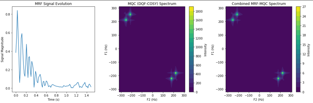
Leave a Reply