
see: https://www.kaggie.com/a-deep-dive-into-vision-transformers-and-clip/
(note, this is only 1 epoch. Certainly a better result would occur with more training.)
import torch
import torch.nn as nn
import torch.optim as optim
import torchvision
import torchvision.transforms as transforms
import matplotlib
matplotlib.use('Agg')
import matplotlib.pyplot as plt
import numpy as np
import seaborn as sns
import pandas as pd
from sklearn.metrics import confusion_matrix, accuracy_score
import json
import os
# Define the ViT model (simplified for brevity)
class ViT(nn.Module):
def __init__(self, num_classes: int = 10, img_size: int = 28, patch_size: in
t = 7, num_layers: int = 6, num_heads: int = 4, embed_dim: int = 64):
super().__init__()
self.patch_size = patch_size
self.embed_dim = embed_dim
self.num_patches = (img_size // patch_size) ** 2
self.patch_embedding = nn.Conv2d(1, embed_dim, kernel_size=patch_size, s
tride=patch_size) # Assuming grayscale images (1 channel)
self.pos_embedding = nn.Parameter(torch.randn(1, self.num_patches + 1, e
mbed_dim)) # +1 for CLS token
self.transformer_encoder = nn.TransformerEncoder(nn.TransformerEncoderLa
yer(embed_dim, num_heads, dim_feedforward=embed_dim*4, batch_first=True), num_la
yers)
self.cls_token = nn.Parameter(torch.randn(1, 1, embed_dim))
self.fc = nn.Linear(embed_dim, num_classes)
def forward(self, x: torch.Tensor) -> torch.Tensor:
# Patchify the image
x = self.patch_embedding(x) # (B, embed_dim, H/P, W/P)
x = x.flatten(2).transpose(1, 2) # (B, num_patches, embed_dim)
# Prepend CLS token
cls_tokens = self.cls_token.expand(x.shape[0], -1, -1)
x = torch.cat((cls_tokens, x), dim=1)
# Add positional embedding
x = x + self.pos_embedding[:, :(x.shape[1]), :]
# Transformer encoder
x = self.transformer_encoder(x)
# Classification head
x = self.fc(x[:, 0]) # Take CLS token for classification
return x
def main():
print("Starting MNIST model training...")
# Device configuration
device = torch.device('cuda' if torch.cuda.is_available() else 'cpu')
print(f"Using device: {device}")
# 1. Download MNIST dataset
transform = transforms.Compose([
transforms.ToTensor(),
transforms.Normalize((0.1307,), (0.3081,)) # Mean and std of MNIST
])
train_dataset = torchvision.datasets.MNIST(root='./data', train=True, downlo
ad=True, transform=transform)
test_dataset = torchvision.datasets.MNIST(root='./data', train=False, downlo
ad=True, transform=transform)
# Use smaller subsets for faster training
subset_size = 50 * 128 # 50 batches * batch_size = 6400 samples
train_dataset = torch.utils.data.Subset(train_dataset, range(subset_size))
test_dataset = torch.utils.data.Subset(test_dataset, range(1000)) #Small tes
t set
batch_size = 128
train_loader = torch.utils.data.DataLoader(train_dataset, batch_size=batch_s
ize, shuffle=True)
test_loader = torch.utils.data.DataLoader(test_dataset, batch_size=batch_siz
e, shuffle=False)
print(f"Downloaded MNIST dataset and created dataloaders.")
# 2. Define the model
model = ViT().to(device)
print(f"Created ViT model: {model}")
# 3. Training loop
criterion = nn.CrossEntropyLoss()
optimizer = optim.Adam(model.parameters(), lr=0.001)
num_epochs = 1
loss_list = []
print(f"Starting training for {num_epochs} epochs...")
for epoch in range(num_epochs):
for i, (images, labels) in enumerate(train_loader):
images = images.to(device)
labels = labels.to(device)
# Forward pass
outputs = model(images)
loss = criterion(outputs, labels)
# Backward and optimize
optimizer.zero_grad()
loss.backward()
optimizer.step()
loss_list.append(loss.item())
if (i+1) % 50 == 0:
print (f'Epoch [{epoch+1}/{num_epochs}], Step [{i+1}/{len(train_
loader)}], Loss: {loss.item():.4f}')
print("Finished training.")
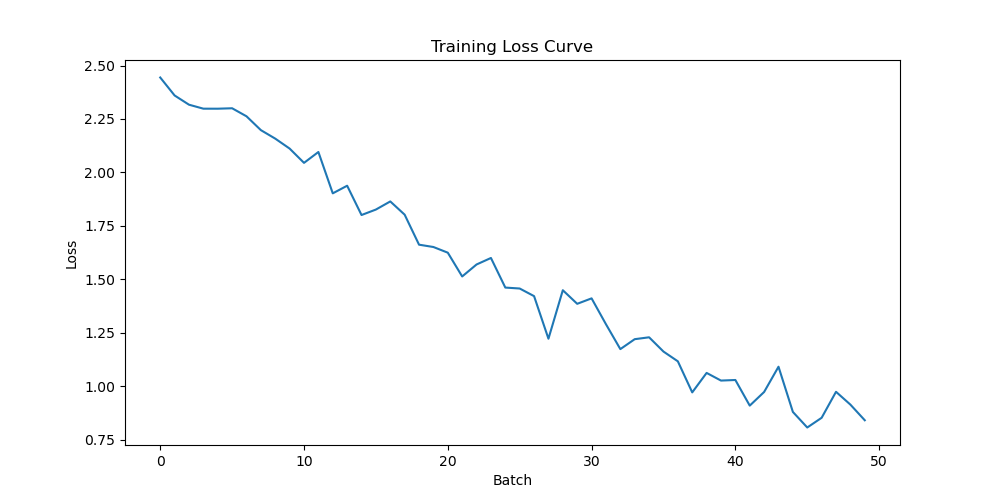
# 4. Generate and save loss curve
plt.figure(figsize=(10, 5))
plt.plot(loss_list)
plt.xlabel('Batch')
plt.ylabel('Loss')
plt.title('Training Loss Curve')
plt.savefig('loss_curve.png')
print("Saved loss curve to loss_curve.png")
# 5. Generate and save metrics
model.eval() # Set model to evaluation mode
all_labels = []
all_predictions = []
with torch.no_grad():
for images, labels in test_loader:
images = images.to(device)
labels = labels.to(device)
outputs = model(images)
_, predicted = torch.max(outputs.data, 1)
all_labels.extend(labels.cpu().numpy())
all_predictions.extend(predicted.cpu().numpy())
accuracy = accuracy_score(all_labels, all_predictions)
final_loss = loss_list[-1]
metrics = {'accuracy': accuracy, 'final_loss': final_loss}
with open('metrics.json', 'w') as f:
json.dump(metrics, f)
print("Saved metrics to metrics.json")
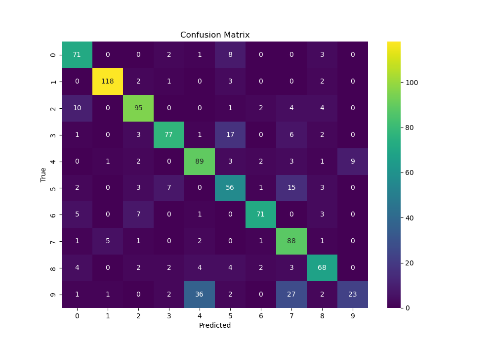
# 6. Generate and save confusion matrix
cm = confusion_matrix(all_labels, all_predictions)
df_cm = pd.DataFrame(cm, index = range(10), columns = range(10))
plt.figure(figsize = (10,7))
sns.heatmap(df_cm, annot=True, fmt='d', cmap='viridis')
plt.xlabel('Predicted')
plt.ylabel('True')
plt.title('Confusion Matrix')
plt.savefig('confusion_matrix.png')
print("Saved confusion matrix to confusion_matrix.png")
if __name__ == "__main__":
if not os.path.exists("./data"):
os.makedirs("./data")
main()Code explanation by Gemini:
This code implements a Vision Transformer (ViT) to classify handwritten digits from the MNIST dataset.
Instead of using traditional Convolutional Neural Networks (CNNs) that look at pixels through sliding windows, this model treats an image like a sequence of text, breaking it into “patches” and using the Transformer architecture (the same tech behind ChatGPT) to understand the relationships between those patches.
1. The ViT Architecture
The class ViT is the heart of the script. Here is how it processes an image:
A. Patchify and Embed
The Transformer can’t “see” a 2D image directly.
patch_embedding: It uses ann.Conv2dwith astrideequal to thepatch_size. This effectively chops a $28 \times 28$ image into $4 \times 4$ grid of patches (each $7 \times 7$ pixels).- Flattening: These patches are flattened into a 1D sequence of vectors.
B. The CLS Token and Positional Embedding
cls_token: A special “Classification” token is added to the start of the sequence. By the end of the layers, this token will hold the “summary” of the entire image.pos_embedding: Since Transformers don’t know the order of the sequence naturally, we add “positional embeddings” so the model knows which patch was in the top-left vs. the bottom-right.
C. The Transformer Encoder
nn.TransformerEncoder: This is a stack of layers that uses Self-Attention. Each patch “looks” at every other patch to determine which parts of the image are most important for identifying the digit.
D. The Head
self.fc: After passing through the encoder, we ignore all the patch outputs and only take the output of the CLS token. This vector is passed to a Linear layer to decide if the digit is $0, 1, 2…9$.
2. The Training Pipeline (main)
The rest of the script handles the “life cycle” of the model:
| Phase | Description |
| Data Prep | Downloads MNIST, normalizes the pixel values, and creates a Subset (6,400 samples) to make training faster for a demonstration. |
| Optimization | Uses Adam optimizer and CrossEntropyLoss (the standard for classification). |
| Training Loop | Feeds images to the model, calculates error (loss), and updates weights using backpropagation. |
| Evaluation | Switches to model.eval() mode to test the model on unseen data without updating weights. |
3. Visualization and Outputs
The script doesn’t just train; it documents the results by saving three files:
loss_curve.png: A line graph showing how the error decreased over time.metrics.json: A text file containing the final accuracy and loss.confusion_matrix.png: A heatmap showing exactly which digits the model confused (e.g., if it often mistook a4for a9).
Key Technical Detail
In the forward pass, notice this line:
Python
x = x + self.pos_embedding[:, :(x.shape[1]), :]
This is a standard “shortcut” to add spatial information. Because the sequence length includes the extra CLS token, the positional embedding is sized num_patches + 1.
Leave a Reply